[Additional Notes:
Latest News, 9 MARCH 2011:
Per FLEX, this problem is now FIXED!!!
Gerald's Email to FlexRadio Customers states, in part:
7 MARCH 2011:Gerald's Email to FlexRadio Customers states, in part:
"Fixed ALC overshoot and corrected leveler gain
target in the transmitter audio signal chain.
These changes have been verified by customers
on air and in the FlexRadio lab using a digital
storage oscilloscope to eliminate overshoot."
The word from Flex is that they've tested a solution which looks very promising.
Also, additional analysis reveals that the overshoot isn't due to Gibbs Phenomena (as I first hypothesized (see below)), but instead I now believe it's because ALC action occurs before the "real" TX signal is converted to I and Q. Shifting a signal's frequency components each by 90 degrees can result in a time-domain signal whose amplitude exceeds that of the original ALC-limited signal, as demonstrated in the graph below:
(Click on image to enlarge)
 Blue Waveform (Sawtooth)
= sin(2πx) + 0.5(sin(2π2x)) + 0.33(sin(2π3x)) + 0.25(sin(2π4x)) + 0.2(sin(2π5x)) + 0.167(sin(2π6x))
Red Waveform (Sawtooth w/components shifted 90o)
= cos(2πx) + 0.5(cos(2π2x)) + 0.33(cos(2π3x)) + 0.25(cos(2π4x)) + 0.2(cos(2π5x)) + 0.167(cos(2π6x))
= cos(2πx) + 0.5(cos(2π2x)) + 0.33(cos(2π3x)) + 0.25(cos(2π4x)) + 0.2(cos(2π5x)) + 0.167(cos(2π6x))
[By the way, despite the way it looks, the Red waveform does not have a DC shift. If you examine the equation from which this graph was generated, you'll note that there are only cosine terms in the equation, and that there is no "constant" term, which would represent a DC shift.]
Imagine that the Blue waveform, being our TX signal, had been "normalized" by ALC operation to have a maximum amplitude of 1.0 (i.e. divide all the values in the graph above by 1.5 so that the Blue waveform has a Vpeak of 1.0). The Red waveform, which is the TX signal with its frequency components shifted by 90 degrees, would have a peak amplitude exceeding 1.0 if its components were also normalized by the same amount (divided by 1.5).
And so, to properly limit the signal, ALC must be applied after the conversion from real to complex data. Which, coincidentally, my fix (described below) does.
Interestingly, if a Triangle-wave's components are phase-shifted by 90 degrees, the resultant signal has an amplitude less than the original's amplitude. Which correlates nicely with our observation that we don't see overshoot with a Triangle wave as our signal, but we do if the signal is a Sawtooth wave.
Below is a plot from a MATLAB simulation. It shows the following:
o Audio sawtooth waveform, fundamental frequency of 200 Hz and band-limited between 200 and 2400 Hz, and of peak amplitude = 1.
o Audio sinewave (200 Hz) of peak amplitude = 1 (will be used as reference).
o The original audio sawtooth waveform, but now with its frequency components shifted by -90 degrees.
o RF Output, LSB, with 200 Hz tone modulation overlayed (for comparison) on RF LSB waveform with sawtooth modulation (and both shifted +4 to that, when plotted, they won't cover our original audio waveforms).
o RF Output, USB, with 200 Hz tone modulation overlayed (for comparison) on RF USB waveform with sawtooth modulation (and both shifted -4 to that, when plotted, they won't cover our original audio waveforms).
(Click on image to enlarge)

Note that the Sawtooth's RF waveform has a peak of 1.759 compared to the 200 Hz Tone's RF peak of 1.000, even though both the Sawtooth and the Tone have the same peak audio amplitude of 1.0. Therefore, if a transmitter were adjusted so that, when driven with the tone, its output was 100 watts (peak), then if the transmitter were driven with a Sawtooth of equal amplitude to the tone, its peak RF output would be 310 watts (i.e. an increase of 4.9 dB in peak power).
And here is the MATLAB code for the simulation, for reference:
clc
% k6jca SSB Modulation Example
%
% Let audio be a 200Hz Sawtooth, of maximum amplitude 1 and band-limited
% between 200 and 2400 Hz.
% Plot 10K points
for inc = 1:100000
% time tick represents 0.1us.
% So total simulation time will be 1e-7*1e5 = 10ms. (2 cycles of 200Hz)
t = (inc-1)*0.0000001;
x(inc) = t;
% in-phase sawtooth waveform with frequency components
% from 200 to 2400 Hz. And scaled by 1.725 so that peak amplitude is 1.
i(inc) = (sin(2*pi()*200*t)+ 0.5*(sin(2*2*pi()*200*t))...
+ 0.33*(sin(3*2*pi()*200*t)) + 0.25*(sin(4*2*pi()*200*t))...
+ 0.2*(sin(5*2*pi()*200*t)) + 0.167*(sin(6*2*pi()*200*t))...
+ 0.1429*(sin(7*2*pi()*200*t)) + 0.125*(sin(8*2*pi()*200*t))...
+ 0.1111*(sin(9*2*pi()*200*t)) + 0.1*(sin(10*2*pi()*200*t))...
+ 0.0909091*(sin(11*2*pi()*200*t))...
+ 0.083333*(sin(12*2*pi()*200*t)))/1.7275;
% quadrature generated by shifting in-phase with a 90 degree delay
% (i.e. subtract pi/2)
q(inc) = (sin(2*pi()*200*t-pi()/2)+ 0.5*(sin(2*2*pi()*200*t-pi()/2))...
+ 0.33*(sin(3*2*pi()*200*t-pi()/2)) + 0.25*(sin(4*2*pi()*200*t-pi()/2))...
+ 0.2*(sin(5*2*pi()*200*t-pi()/2)) + 0.167*(sin(6*2*pi()*200*t-pi()/2))...
+ 0.1429*(sin(7*2*pi()*200*t-pi()/2)) + 0.125*(sin(8*2*pi()*200*t-pi()/2))...
+ 0.1111*(sin(9*2*pi()*200*t-pi()/2)) + 0.1*(sin(10*2*pi()*200*t-pi()/2))...
+ 0.0909091*(sin(11*2*pi()*200*t-pi()/2))...
+ 0.083333*(sin(12*2*pi()*200*t-pi()/2)))/1.7275;
% For reference (and comparison) generate a 200 Hz tone of peak ampitude 1
i_tone_200(inc) = sin(2*pi()*200*t);
q_tone_200(inc) = sin(2*pi()*200*t - pi()/2);
% Now let's generate our RF. First, in-phase. Frequency is 1 MHz.
rf_i(inc) = cos(2*pi()*1e6*t);
% quadrature by delaying rf by 90 degrees (subtract pi/2);
rf_q(inc) = cos(2*pi()*1e6*t - pi()/2);
% Now let's calculate out in-phase and quadrature channels...
in_phase(inc) = i(inc) * rf_i(inc);
quad(inc) = q(inc) * rf_q(inc);
% ...and then add or subtract them to make LSB and USB
lsb(inc) = in_phase(inc) + quad(inc);
usb(inc) = in_phase(inc) - quad(inc);
% For reference, let's also make LSB and USB using the 200 Hz tone,
% so that we can see if its peak RF differs from the sawtooth's
% peak RF
lsb_tone(inc) = i_tone_200(inc) * rf_i(inc) + q_tone_200(inc) * rf_q(inc);
usb_tone(inc) = i_tone_200(inc) * rf_i(inc) - q_tone_200(inc) * rf_q(inc);
end
top = max(i);
top_q = max(abs(q));
top_lsb = max(abs(lsb));
top_tone = max(abs(lsb_tone));
figure
plot(x,i,x,q,x,i_tone_200,x,lsb_tone+4,x,lsb+4,x,usb_tone-4,x,usb-4);
grid on;
legend('sawtooth (input)','input shifted -90 degrees','200Hz Tone (Reference)','LSB of 200Hz Tone','LSB of sawtooth','USB of 200Hz Tone', 'USB of sawtooth');
My original post is below...]
On the topic of TX overshoot with the Flex 5000...
Last summer a friend of mine mentioned that he was having a problem with PowerSDR and his Alpha amplifier -- it looked to him as though RF overshoots at the Alpha's input were causing it to shut down, and these shutdowns were occurring frequently enough to really annoy him.
I decided to do a bit of investigation. When I looked at the RF envelope from my Flex 5000, I saw overshoots with my 1.18 Console. Thinking that the problem might be related to the software revision, I downloaded the 2.0.7 PowerSDR Console and ran my tests again. Below are snapshots of the OUTPUT RF waveform from my 5000 using the 2.0.7 console.
Oscilloscope is my Tek 2445 that I use to monitor my transmit RF (via an RF-sampler). The two horizontal cursors you see on its CRT mark the peak-to-peak level of the RF signal when the 5000 is in TUN mode and the Tune level is set to 10 watts.
For the following snapshots, PowerSDR is set to:
- Freq: 3.863 MHz
- Mode: LSB
- Drive: 10
- Leveler: Disabled
- TX EQ: OFF
- DX: OFF
- CPDR: OFF
- DEXP: OFF
Anyone can try this experiment with these setting. Here are my results:
First, two nicely behaving waveforms:

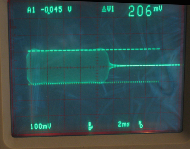 Notice how the peaks don't exceed (by much) 10 watts?
But look at these next two. Yikes!


The four snapshots are:
- Triangle waveform from internal internal software Transmit generator. Looks great!
- Pulse, from the internal software Transmit generator (at its default settings for Pulse mode). Looks great!
- Sawtooth waveform from the internal software Transmit generator. Yikes -- it greatly exceeds the 10-watt cursors! Peak power is 49 watts on my LP-100 power meter, yet DRIVE is set to 10 watts.
- My voice, saying "Ahhh" loudly into microphone. Yikes again! Peak power is about 40-50 watts on my LP-100 power meter, yet DRIVE is set to 10 watts.
In AM mode, the sawtooth (as modulation) looks exactly as it should, so I don't believe the issue with the sawtooth is that it's somehow "broken."
I thought I'd experiment with the code a bit and see if I could gain further insight...
First, I experimented with the ALC code itself, as my first suspicion was that the overshoot was due to the non-zero attack time. But nope, that wasn't it. I changed the attack time to 0 (so that the ALC was a true peak-detector, and not one with a non-zero attack time), and it made no appreciable difference in the gross overshoots experienced by voice or sawtooth SSB modulation.
I then played around with the location of the ALC algorithm, and the results are very interesting. If the ALC code is prior to the filter_OvSv routine (as it is in the version of code I'm using (v1.18.4) as well as in the SVN 3862 code that I downloaded), then both Voice and Sawtooth waveforms grossly overshoot the target power, per the photos above. In other words, the current ALC code in its current position, in either my console (1.18.4) or in the 2.0.7 console, does not properly limit the output RF for certain waveforms.
However, if I move the ALC code to just after the filter_OvSv routine (and change the buffers used for ALC in newDttSPAGC from buf.i to buf.o), then there is minimal overshoot for all waveforms (Tone, Triangle, Sawtooth, and Voice), and their peaks are all near the target power. In other words, the output RF looks beautiful. [Note: I wasn't able to test the PULSE waveform, because my 1.18 version of the console doesn't have PULSE as one of the options for the test generator].
I'll make a wild guess that the overshoot is due to the bandpass filtering in filter_OvSv and thus similar to Gibb's phenomena. But this is just a guess. Conceptually, it makes sense to me that the ALC processing should be as late in the processing chain as possible, and moving it to just after filter_OvSv seems to be a better place for it than prior filter_OvSv. However, I'll be the first to admit that I don't know what the ramifications are of doing this. Are other problems introduced? I don't know.


No comments:
Post a Comment